5. LUMFILE (Lumet file analysis)

5.1. Introduction

LUMFILE is the module dedicated to the analysis of laser ultrasonic data obtained from the Laser Ultrasonics sensor.

The Graphical user interface of the module LUMFILE is shown in the figure below. The module is composed of 3 parts, i.e. i) a control display on the left hand side ii) a graphic display region right hand side and iii) a setting window dialog.

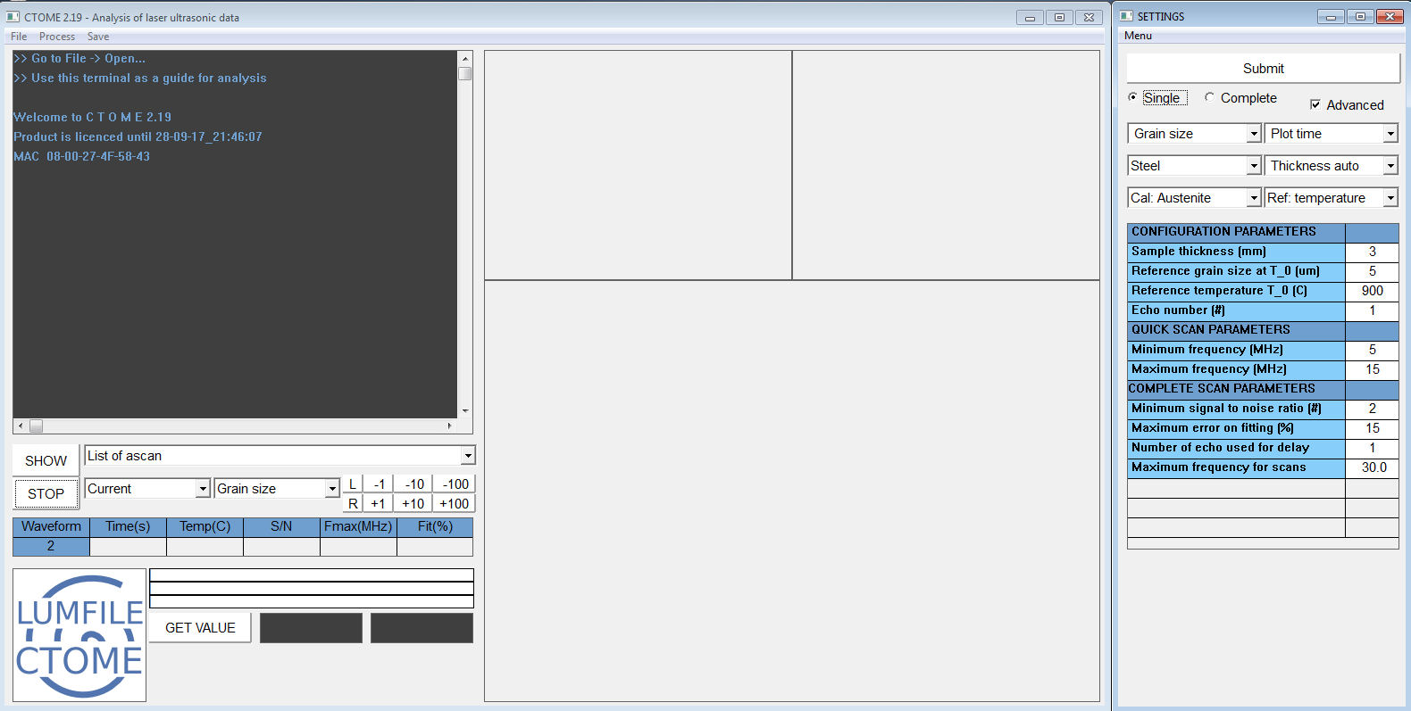
The following section defines the name of the parameter and their function, the options available in each drop-down and the action of each button and scale bars.

5.2. Software parameters

This part defines the different adjustable parameters and settings of the LUMFILE module.

5.2.1. Main Window

5.2.1.1. Top menu bar

File/Open:Start the wizard to load file from the LUMFILE directory. File must be placed in a folder contained in the LUMFILE directory. For one tests, the three files must be present in the folder (1-ASCAN, 2-DT file 3-D file) Process/Setting:  Open the setting dialog. Process/Fraction transformed:  Open the dialog to configure the fraction transformed calculation. Process/Recrystallization:  Open the dialog to configure the recrystallization fraction calculation. Save/Single scan results:  Save the results of a single scan into an ASCII output file. Save/Raw Waveform:  Export a raw or unfiltered waveform. The file contains two columns with time(us) and Amplitude (V) Save/Filtered Waveform:  Export a processed or filtered waveform i. The file contains two columns with time(us) and Amplitude (V) Save/Raw Waveform Spectrum:  Export a raw or unfiltered waveform spectrum. The file contains two columns with frequency(MHz) and magnitude of the Fourier transform of the waveform. Save/Raw Waveform Spectrum:  Export a raw or unfiltered waveform spectrum. The file contains two columns with frequency(MHz) and magnitude of the Fourier transform of the waveform. Save/Attenuation spectrum:  Open a dialog for specific operation on the attenuation spectrum, averaging, fitting and exporting.

5.2.1.2. Terminal

The output terminal is used for multiple purpose, it display tips, currents settings, and status of the analysis.

5.2.1.3. Buttons

SHOW:Shows the file selected on the combobox listing the current files loaded. STOP:Interrupt a scan. GET VALUE:A value can be obtained by clicking this button button and then click on the appropriate area of the graph to get the coordinate of the point. L:Move to the left side of the scale bar R:Move to the right side of the scale bar +1:Add 1 to the value of the scale bar. This button is only active if their is at least 1 more value to display after the current value. +10:Add 10 to the value of the scale bar. This button is only active if their is at least 10 more values to display after the current value. +100:Add 100 to the value of the scale bar. This button is only active if their is at least 100 more values to display after the current value. -1:Remove 1 to the value of the scale bar. This button is only active if their is at least 1 value to display before the current value. -10:Remove 10 to the value of the scale bar. This button is only active if their is at least 10 values to display before the current value. -100:Remove 100 to the value of the scale bar. This button is only active if their is at least 100 values to display before the current value.

5.2.1.4. Combobox

1. File selection combobox, display a list of the file selected for analysis.

2. Waveform graphs: Display a list of options for the graph located in the top raw and left hand side. The properties display here are attributed to individual waveforms. The available option are:

   • Current:: Display the current waveform
   • Reference:: Display the reference waveform
   • Delay:: Display the cross correlation function
   • Echo:: Display the amplitude spectrum of selected echoes
   • Noise:: Display the waveform spectrum and the RMS(noise)
   • Attenuation:: Display the attenuation spectrum

3. Metallurgical process graphs: Display a list of options for the graph located in the bottom raw. The properties display here are attributed to whole tests. The available options are:

   • Thickness:: Display the evolution of the relative change in thickness of the sample during the test.
   • Noise:: Display the evolution of the noise level during the test.
   • X Correlation:: Display the evolution of the amplitude of the cross correlation function during the test.
   • Velocity:: Display the evolution of the velocity during the test.
   • Signal/Noise:: Display the evolution of the signal to noise ratio during the test.
   • Bandwidth:: Display the evolution of the available bandwidth during the test.
   • Standard Error:: Display the evolution of the goodness of the least square regression applied to the attenuation spectrum.
   • Attenuation:: Display the evolution of the attenuation at 4 frequencies located within the selected bandwidth.
   • Grain size Variable:  : Display the evolution of the attenuation parameter related to the mean grain size in the sample.
   • Grain size:: Display the evolution of the mean grain during the test.
   • Fraction Transformed:  : Display the evolution of the fraction transformed during the test.
   • Fraction Recrystallized:  : Display the evolution of the fraction recrystallized during the test.

5.2.1.5. Table

The table shows the current waveform, current temperature and time as well as the value of the signal/noise ratio, maximum frequency for the current waveform and the goodness of the non-linear least square regression applied to the attenuation spectrum. A color code indicates if the waveform have pass a series of acceptance criteria. Green means that it has pass the test and red means that the waveform will be rejected.

5.2.1.6. Progress bars

Three progress bar are integrated:

1. The top progress bar indicates the progress of an individual scan
2. The middle progress bar indicates the progress of a multiple or complete scanning sequence for an individual ascan file.
3. the bottom progress bar indicates the progress of a multiple scan on multiple files.

5.2.1.7. Hidden panel

By extending manually the main window to the right, number of scale bar become accessible. They are used to zoom and adjusts ranges of axes in the figure.

WAVEFORM, Xmin:Set the minimum value for the X axis of the current waveform and reference waveform graph in microsecond. WAVEFORM, Xmax:Set the maximum value for the X axis of the current waveform and reference waveform graph in microsecond. WAVEFORM Y scale:  Set the scaling factor for the Y axis of the current waveform and reference waveform graph, in percent. SPECTRUM Xmin:Set the minimum value for the X axis of the Waveform spectrum graph in MHz. SPECTRUM Xmax:Set the maximum value for the X axis of the Waveform spectrum graph in MHz. SPECTRUM Yscale:  Set the scaling factor for the Y axis of the attenuation spectrum graph. Zoom in Graph (%):  Set the scaling factor for the zoom applied on the bottom graph showing i) Attenuation at single frequency, ii) Velocity, iii) Grain size iiii) Fraction

In addition are the following options:

1. Sync Auto:: If selected, the software conduct a step of automatic detection of the optimum threshold.
2. Set Fmin:: If selected the user can enter the value of the minimum frequency to be used in the non-linear least square regression applied to the attenuation spectrum. It is recommended not to play with this option.
3. Func_ref:: This option is used only for academic purposes.

5.2.2. Setting Dialog

5.2.2.1. Top menu bar

Menu/Save current parameters as default:  Save the current setting as default value. Menu/Reset default parameters:  Recover the default value from first install.

5.2.2.2. Buttons and check boxes

SUBMIT:Start a scan using the current setting Advanced:Display the advanced parameter in the setting table. Single:Select single scan using the parameter in the setting table. It will only generate one scan using selected Fmin and Fmax. Complete:Select complete scan using the parameter in the setting table. It will generate a number of scan by varying the value for Fmin and Fmax and reporting the results into a pdf automatically generated.

5.2.2.3. Table

CONFIGURATION PARAMETERS:   Sample thickness (mm):  Initial sample thickness at room temperature. Direction parallel to the wave propagation. (Default value is 3 mm) Reference grain size at T_0 (um):  Known metallographic grain size at the reference temperature. Reference temperature T_0 (C):  Reference temperature. Echo number (#):  Echo number selected for the evaluation of the attenuation spectrum. In the Single Echo method, the attenuation is calculated from the ratio of the amplitude spectrum of the echo number given by Ref.Echo. in the Reference waveform and in the current waveform. In the Two echoes method, the attenuation is calculated from the ratio of the amplitude spectrum of the echo number given by Ref.Echo. and Ref.Echo.+1 in the current waveform. QUICK SCAN PARAMETERS:   Minimum frequency (MHz):  Lowest frequency considered in the non-linear regression applied to the attenuation spectrum. Maximum frequency (MHz):  Maximum frequency selected for the analysis. COMPLETE SCAN PARAMETERS:   Minimum signal to noise ratio (#):  Minimum signal to noise ratio accepted for the acceptance and rejection of the waveform. Maximum error on fitting (%):  Highest frequency considered in the non-linear regression applied to the attenuation spectrum. Number of echo used for delay:  Specifies the number of echo between the Echo number (#) and the second echo in the two echo method used for velocity measurements. Maximum frequency for scans:  Specifies the maximum frequency that needs to be scan during a complete scan experiments. OTHER PARAMETERS:   Sample width of diameter (mm):  Specified the width of the sample or the initial sample size to be taken for the dilatometry measurement. Direction perpendicular to the wave propagation. (Default value is 10 mm) Reference Waveform Number:  : Waveform number selected for the application of the Single Echo method. This waveform will be selected from the reference ascan file as the reference waveform.

5.2.2.4. Combobox

1. Mode selection

   • Elastic modulus: Select the Two Echo method for the evaluation of the velocity and attenuation. The same waveform is used for the selection of the reference and current echo.
   • Grain size: Select the Single Echo method for the evaluation of the velocity and attenuation. Different waveforms are used for the selection of the reference and current echo.

2. Material selection

   • Steel
   • Aluminium
   • Copper
   • Aust SS
   • Niobium
   • Titanium (hcp)
   • Titanium (bcc)
   • Cobalt (fcc)

3. Axis selection

   • Plot time
   • Plot temperature

4. Thickness

   • Thickness auto : Specify that no information are available for the variation of the thickness of the sample with temperature. The model parameter for the selected material will be used instead.
   • Dilatometer : Specify that some dilation measurement are conducted on the width of the sample during the LUMet testing and are available for the variation of the thickness of the sample with temperature. Isotropic assumption is considered between the variation measured in the width and in the thickness of the sample.

5. Calibration

   • Cal: Autenite: Specify that the austenite calibration for low alloy steel method will be used for the evaluation of grain size from the attenuation measurement.
   • Cal: Cobalt : Specify that the Cobalt calibration will be used for the evaluation of grain size from the attenuation measurement.

6. Reference

   • Ref. Temperature
   • Ref. Time

5.3. Methodology:

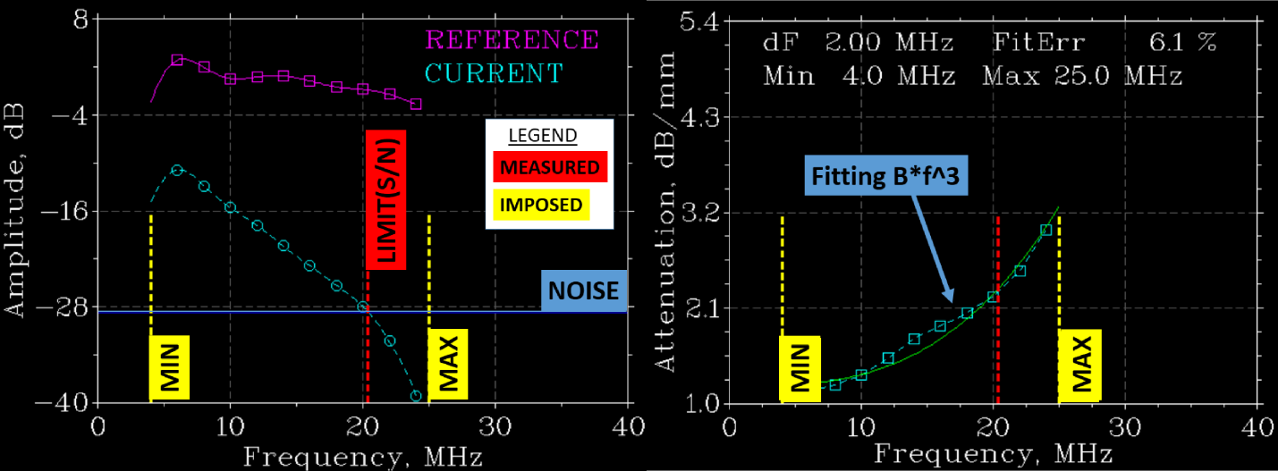
Spectral analysis is conducted on the pressure wave measured after the pulse travels once and twice through the sample. For sake of example, this report includes the results obtained with the second echo. Figure below (left) depicts the amplitude of a current and reference echo with respect to the ultrasound frequency. The minimum frequency and maximum frequency are setting the lower and upper bound for the non-linear regression applied to the attenuation spectrum shown in Figure 3 (Right). The attenuation spectrum is calculated by the ratio of the amplitude spectrum of the current and reference echoes. It is expressed in dB per unit of length. The fit applied to the attenuation spectrum follows the methodology described in detail in the literature and the grain size is deduced from the parameter b by the application of a grain size calibration available for low alloyed steel.

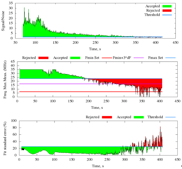
During the analysis, each laser ultrasound measurement is submitted to a series of three selection criteria, 1) Signal to noise, 2) Measured bandwidth 3) Quality of the fit. The figure below illustrate the evolution of the three criteria for a selected test. For each of the criteria, a threshold is set to either accept or reject the particular waveform. If all three criteria are satisfied the grain size parameter b is given a confidence index calculated by comparing how far from the threshold value each criteria was satisfied. (Detail on this procedure is reported in the following parts). The values selected for the threshold limits are identical for all the analysi presented in the present report and indicated in the pdf report.

A priori, the optimum value for the min and max value of the frequency bandwidth is not known and strongly depends on various factors such as temperature, grain size and may be affected by the surface conditions. A Table included in the final report shows the total number of scan conducted for the analysis. The minimum frequency ranges from 3.3 to 6.7 MHz and the maximum frequency ranges from 8.3 to 35 MHz. For a given value of the minimum frequency, the smallest value for the maximum frequency is set so that the bandwidth is at least 3 times the resolution in frequency.

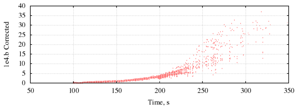
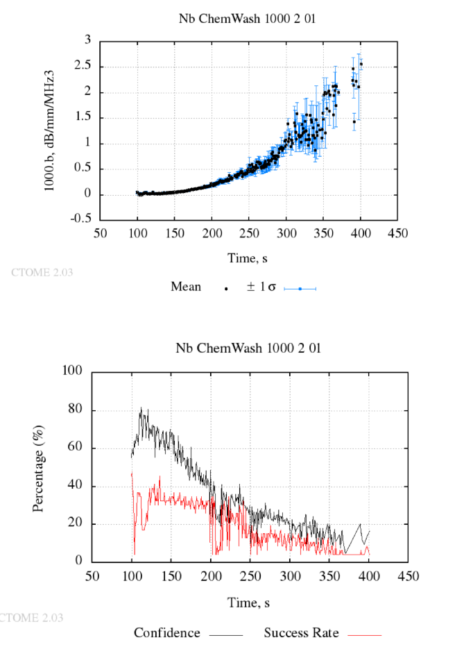
Once the scans are completed, the grain size parameters b measured for each bandwidth is compiled is a master plot as depicted in Figure 5. The average value of the grain size parameter as well as the standard deviation is weighted by the confidence index obtained at each scan (Figure 6). Detail on this procedure is provided in the joined pdf.

5.4. Analysis criterion

The parameters b (grain size parameter) is calculated by the processing of the ultrasound waveforms measured during the heat treatment cycle. The analysis is divided in several steps. At each step, the waveform (representing the signal measured a specific time of the treatment) is accepted or rejected accordingly to 5 criteria. The testing sequence verifies i) that amount of light collected is sufficient, ii) that the signal to noise ratio is acceptable, iii) that the selected bandwidth, min and max frequency considered are resolved given the signal to noise conditions, iv) that the quality (or standard error) of the least square fitting on the attenuation spectrum is acceptable and v) that the measurement of grain size parameter falls in the range of applicability for the selected grain size calibration. Each of these test contains a setting parameter to adjust the limits and threshold for each measured quantity. The notions of confidence index is introduced for each of the criteria. It is aimed to evaluate how successfully a measurement pass a tests. The details on the evaluation of the confidence index for each criteria is reviewed in the following part.

5.4.1. Waveform Synchronization

The first steps of the analysis aims to accurately synchronize each waveform with one another. The time at the onset of the generation is determined in order to evaluated the level of the laser noise (prior to generation). The criteria is based on the definition of a threshold amplitude. The time at the bang of generation is the time where the amplitude of the signal becomes higher than the selected threshold amplitude. The value for the threshold amplitude is not known a priori for each waveform and varies slightly from sample to sample depending on the surface reflectivity and overall quality of the signal. A dedicated pre-processing steps is used to find the optimum threshold value that will successful synchronized the largest number of waveforms.

5.4.2. Light collected

Most sensors allows for the evaluation of the quantity of light collected in the detector. The light collected criterion is introduced to verify that the quantity of light is larger than a pre-determined threshold. The information is also used to normalize the amplitude of waveform with the amount of light collected in the laser probe. This option requires appropriate settings on the PreTrigLength and DelayIntegration as well as the addition of a *.pwl file in the selected directory. (Ask system admin)

5.4.3. Signal to Noise and Fmax

The signal to noise ratio is evaluated at each analysis. It is the ratio of the rms(echo signal) to the rms(laserNoise) measured prior to the bang of generation. It is estimated both in the frequency domain and in the time domain. The rms value measured in the frequency domain determines the maximum frequency resolved for the calculation of the the grain size parameter. The signal to noise ratio is defined as \Theta^{noise}_{\varphi} and the maximum frequency resolved F_max_true.

1. In the time domain (for the signal/noise ratio):

• signal = rms(echo_current(t)),
• noise = rms(noise(t)), mesured before the generation

2. In the frequency domain (for the F_max_true) :

• signal(f) = echo_current(f),
• noise = rms(noise(f))

F_max_true is the frequency at which the amplitude spectrum of the echo signal is lower than the amplitude of the noise, such as Ampl.signal(f)/noise(f) < S/N.

The confidence index on signal to noise ratio \omega^{Noise}_{\varphi} is calculated as in (1)

(1)\omega^{Noise}_{\varphi} = \frac{\Theta^{Noise}_{\varphi}}{\Theta^{noise}_{C}(\alpha -1)}+\frac{1}{1-\alpha}

In (1), \alpha = 10.0 is the severity factor. The confidence index on signal/noise ratio \omega^{noise}_{\varphi} is set to 1 if \Theta^{noise}_{\varphi} > \alpha*\Theta^{noise}_{C}. It is set to 0 if \Theta^{noise}_{\varphi} < \Theta^{noise}_{C}

• Minium signal/noise ratio \Theta^{noise}_{C} = 1.000

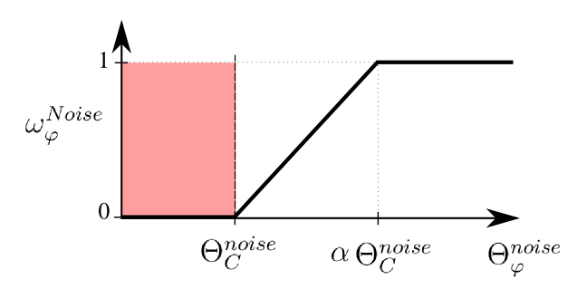
Schematics of the rejection tolerance criteria for the signal to noise

5.4.4. Goodness of attenuation fit

The standard error \Theta^{Fit}_{\varphi} expressed for the grain size parameters (fitting parameter) is evaluated with the algorithms available in the software Gnuplot using the variance-covariance matrix in a similar way to the method used for determining the standard errors in a linear least-square fitting problem * Frequency domain: att(f) = a+b*f^n. * Parameter b_measured = b +/- delta_b(standard error).

The confidence index on the goodness of the fit \omega^{Fit}_{\varphi} is calculated as in (2)

(2)\omega^{Fit}_{\varphi} = -\frac{\Theta^{Fit}_{\varphi}}{\Theta^{Fit}_{C}} + 1

The index \omega^{Fit}_{\varphi} is 0 if \Theta^{Fit}_{\varphi} > \Theta^{Fit}_{C}

• Minium fit error (%) \Theta^{Fit}_{C} = 15.000

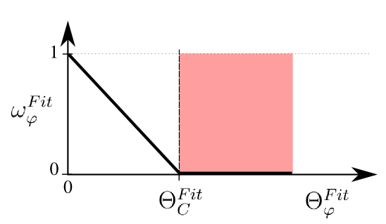
Schematics of the rejection tolerance criteria for the goodness on the attenuation fit.

5.4.5. Range of calibration

Calculate if the fit parameter b is in the range of the available grain size calibration. Alarm is triggered if the parameter is outside the range

The confidence index on this criteria follows a rectangular windows, i.e. 1 if the parameteris contained into the range of calibration and 0 if it is outside the range

5.4.6. Combined confidence per scan

The grain size parameter is calculated by fitting the attenuation spectrum of a selected echo between a minimum frequency and a maximum frequency, i.e. bandwidth. The selection of which echo and what range of frequency or bandwidth should be selected is not known a priori and can influence the end results. Therefore, the process of analysis consist on scanning a range of bandwidth and/or echo (optionally in the program) and to determine the confidence indexesfor each conditions. The confidence index is normalized and is described for each criterion in their own sections above. The combined confidence index per scan \omega^{i}_{\varphi} is then defined by the arithmetic average of the confidence index obtained for the criteria on signal to noise \omega^{Noise}_{\varphi}, and goodness of the fit \omega^{Fit}_{\varphi}. The average confidence index per scan is expressed as shown in (3).

(3)\omega^{i}_{\varphi} = \frac{1}{2}\left ( \omega^{Noise}_{\varphi}+\omega^{Fit}_{\varphi} \right )

5.4.7. Average grain size parameter per waveform

The mean grain size parameter \bar{b}_{\varphi} after a total number of scan N is the average of the grain size parameter b^{i}_{\varphi} obtained at each scan {\varphi} weighted by the confidence index \omega^{i}_{\varphi} as expressed in (4).

(4)\bar{b}_{\varphi}=\frac{\sum_{i=1}^{N}\omega^{i}_{\varphi}b^{i}_{\varphi}}{\sum_{i=1}^{n}\omega^{i}_{\varphi}}

The weighted average standard deviation \sigma_{\varphi} on the mean grain size \bar{b}_{\varphi} is expressed as shown in :eq: stdgrainsize.

(5)\sigma_{\varphi} = \sqrt{\frac{\sum_{i=1}^{n}\omega ^{i}_{\varphi}\left (b^{i}_{\varphi}-\bar{b}_{\varphi} \right )^{2}}{\frac{N-1}{N}\sum_{i=1}^{n}\omega^{i}_{\varphi}}}

Once the average grain size parameter is estimated, the selected calibration is applied to estimate the average grain size for each waveform measured during the thermal cycle.

5.4.8. Average confidence index per waveform

The average confidence index per waveform \bar \omega_{\varphi} is the arithmetic average of the combined confidence index per scan \omega^{i}_{\varphi} as expressed in (6)

(6)\bar \omega_{\varphi} = \frac{\sum_{i=1}^{N}\omega^{i}_{\varphi}}{N}

The standard deviation on the confidence index per waveform \sigma _{\bar \omega_{\varphi}} is expressed in (7)

(7)\sigma _{\bar \omega_{\varphi}} = \sqrt{\frac{\sum_{i=1}^{N}\left ( \omega^{i}_{\varphi} - \bar \omega_{\varphi}\right )^{2}}{N-1}}

5.5. Error estimates

The precision in the measurement of the ultrasonic parameter b (or grain size parameter) was estimated using samples of steels, nickel and cobalt and by computing the distribution of measured values over 60 acquisitions conducted at the same position in the sample at room temperature. A Gaussian distribution was applied to adjust the relative standard deviation σ for each case using a least square fitting method. The standard deviations resulting from the regressions range from 0.020 to 0.028 indicating that the uncertainty in the measurement of the attenuation parameter b, at room temperature, is at least 0.056 (5.6%) with a confidence interval of 95%. Further, b depends on temperature and the uncertainty associated with measurements at high temperatures is determined from the relative square error for a series of data measured up on cooling from high temperature in a sample with constant grain size. The overall uncertainty resulting from this analysis was 10%. When applied to the measurement of grain size, the laser ultrasonics technology requires the construction of a calibration based on the metallographically measured grain size. Many factors are influencing the precision in the determination of the average grain size by metallography as summarized in the ASTM standard E112-12 which include the selected magnification, the ability to properly delineate grain boundaries, the number of grains considered, the total sample area scanned and number of fields of view permitted for the selected magnification as well as the representativeness of the specimens selected and the area chosen for the measurement. Following all guidelines for optimum estimation of the average grain size, and according to the various sources of errors in the procedure, the relative accuracy obtained in this study for the metallographic grain size value is determined to be 15%, i.e. 10% from statistics and 5% from the uncertainty in delineation of grain boundaries. Finally, the uncertainties in the laser ultrasonic grain size resulting from the application of the proposed calibration to any new measurement of the parameter b is estimated by the evaluation of the relative square error on the calibration data. The relative error amounts to about 26%, i.e. laser ultrasonics grain size is measured with a relative precision of ±13%.

5.6. Getting started

5.6.1. Copying the input files into the LUMFILE directory

After an experiments, the raw data must be placed into a dedicated folder placed into the LUMFILE subdirectory of the main work directory. For instance, if the work directory is F:\CTOME\Data\, you must create a new project folder inside the LUMFILE folder within this work directory. For instance, create a new folder and give the name Steel_3mm if you are currently working with steel. Here the thickness of the plate appears in the name of the directory. This makes further analysis more convenient but this is not mandatory. Copy all the three raw files inside this new directory. Their is always 3 files created during a tests, i.e. the ascan file, the dt file and the d file. The new directory should then contain the following:

• F:\CTOME\Data\LUMFILE\Steel_3mm\experience_01.ascan
• F:\CTOME\Data\LUMFILE\Steel_3mm\experience.dt01
• F:\CTOME\Data\LUMFILE\Steel_3mm\experience.d01

You can create as many project folder as you want and conserve all you data organized into the LUMFILE folder.

5.6.2. Loading the input file into the LUMFILE software

• Start the LUMFILE software
• Press File/open to open the file import wizard.
• Select the project folder into which you LUMet+Gleeble data are stored and press OK.
• Select one or multiple files. You can also choose a reference file by enlarging the dialog window to the right. If you don’t select any reference file, the reference state will need to be defined from the setting dialog.

Press OK when you have correctly selected the files you wish to load in LUMFILE.

5.7. Tutorials and step by steps

5.7.1. Evaluation of austenite grain size in STEEL

5.7.1.1. Conducting the test

-STEP 1: Install the sample between the jaws of the gleeble by adjusting the angle to 90 degree of the laser beam.

-STEP 2: Measure a series of waveform in a reference sample having small grain size of ferrite. Ideally, one can consider that a sample with a mean grain size lower than 5 μm is good for the reference sample. The reference sample must have the same geometry as the sample in which the austenite grain size will be measured. The good thing is that once you have this reference signal, it will be suitable for all measurement of grain size conducted in sample having same geometry. In addition, the measurement of the reference must be conducted in the same atmosphere as the subsequent test will be conducted; i.e. vacuum or furnace gas will provide different reference signal. Generally, it is good to acquire about 50 waveforms in this reference sample so as to further benefit for some waveform averaging optimization in the post processing steps.

-STEP 3: Conduct the heat treatment cycle by distributing at most 600 waveforms in the temperature range of interest. One must try to limit the total number of pulses generated at the same position so as to avoid extensive surface damage that could result in a decrease in the signal to noise ratio.

-STEP 4: Once the tests are completed, one must collects the following 6 files and place them into one single folder for post processing with the CTOME software. (Reference signal : Ascan file, DT file, and d0 file; Current signal: Ascan file, DT file and d0 file) The reference file is optional.

5.7.1.2. Analyzing the data

For this example, a test conducted on a 1018 steel is used. It consists on a rapid heating at a rate of 100 ° C/s up to a temperature 1050 ° C followed by a holding for 5 min at this temperature. Laser ultrasonics signal are captured during the entire duration of the holding at high temperature.

At the end of the test, the user must collect three different files. The ascan must be copied from the LUMet computer. The DT file and the D file is copied from the Gleeble computer.

1. Start the software LUMFILE and Load the current file using the file dialog from the File/Open menu. Select one or more than one ascan file. Up to 10 ascan can be loaded simultaneously. Select a reference file if needed. This is optional. If no reference file is selected, then the reference state is defined from the setting dialog.
2. Once the file is done loading, select the methodology grain size from the appropriate combo box and check Complete scan. Indicate the thickness of the sample and the material tested and choose the desired calibration. If you have measured dilation in the width of the sample during the LUMet tests, indicate the initial width of the sample and select dilatometer instead of thickness auto from the appropriate combobox
3. Define the reference state for this sample. Often in steel, it is common to consider that the grain size is small at the end of the austenite formation. Therefore, the default value are D_0 = 5 um at T_0 = 900C. If you have selected a reference, their is no need to define the reference state. Simply indicate the Reference waveform number. Often, the reference file is acquired at room temperature in a sample with small grain size and with optimum conditions for the light collection on the detector. The waveform 5 is selected by default.
4. Select the echo number for the complete scan. Echo 1 or 2 usually are working fine. For thin sample, it s better to use number 2 or 3 as the bang of generation may affect the frequency content of the first couple of microseconds in the waveform.
5. Submit the scan for analysis. The results will be summarized into a pdf file and all process data will have been saved in a specific folder with the project name given to the complete scan.

5.7.2. Measurement of austenite decomposition in steel

5.7.2.1. Conducting the test

-STEP 1: Install the sample between the jaws of the gleeble by adjusting the angle to 90 degree of the laser beam.

-STEP 2: Conduct the heat treatment cycle by distributing about 800 pulses during the heating and cooling step of the treatment.

-STEP3: Collect the 3 files for this measurement (ASCAN file DT file and D0 file) and place them into a dedicated folder for analysis with the LUMFILE module of the CTOME software.

5.7.2.2. Analyzing the data

The following procedure provide a step by step manual on how to use the software LUMFILE to evaluate the kinetics of the austenite decomposition from a set of waveform measured during continuous cooling.

For this type of test, the lumet signal must be monitored during heating and cooling, or only during cooling of the alloy.

At the end of the test, the user must collect three different files. The ascan must be copied from the LUMet computer. The DT file and the D file is copied from the Gleeble computer. All three files must be placed into the project folder as indicated in the section 4.3.

1. Start the software LUMFILE and Load the current file using the file dialog from the File/Open menu. Select one or more than one ascan file. Up to 10 ascan files can be loaded simultaneously.
2. Once the file is done loading, select the methodology Elastic Modulus from the appropriate combo box, this will switch to single scan. Indicate the thickness of the sample and the material tested and choose the desired calibration. If you have measured dilation in the width of the sample during the LUMet tests, indicate the initial width of the sample and select dilatometer instead of thickness auto from the appropriate combobox
3. Select the echo number for the single scan. Echo 1 or 2 usually are working fine. For thin sample, it s better to use number 2 or 3 as the bang of generation may affect the frequency content of the first couple of microseconds in the waveform. You can also click on advanced and select the position of the second echo.
4. Submit the scan for analysis. The results will be available by showing velocity in the appropiate combox from the main window.
5. Once the calculation is completed and that you have calculated the entire velocity curve upon heating and cooling, open the calculation windows from the menu Process > Fraction transformed (Velocity)

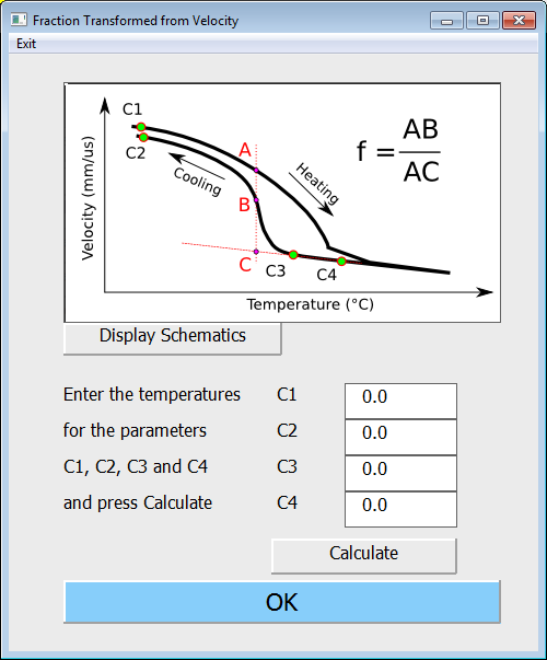
The calculation can be done after entering the four following coefficients.

C1 (C):Temperature used in the evaluation of the austenite fraction transformed from velocity measurement. This parameter is used to offset the entire velocity curve according to the Model velocity for this material at this temperature. It must be included in a temperature range where some velocity measurements are available upon heating. An appropriate choice for this parameter is often the lowest temperature measured upon heating. C2 (C):Temperature used in the evaluation of the austenite fraction transformed from velocity measurement. This parameter is used to offset the cooling portion of the velocity curve according to the velocity measured upon heating at this temperature. This allows the software to compensate for a different velocity upon heating and cooling in case large texture change are associated with the austenite formation. It must be included in a temperature range where some velocity measurements are available upon cooling. An appropriate choice for this parameter is often the lowest temperature measured upon cooling. C3 (C):Temperature used in the evaluation of the austenite fraction transformed from velocity measurement. Low bound of the linear fit applied in the evolution of velocity measured for austenite upon cooling.

C4 (C):

Temperature used in the evaluation of the austenite fraction transformed from velocity measurement. High bound of the linear fit applied in the evolution of velocity measured for austenite upon cooling.

Once the values are entered in the appropriate boxes, click the button CALCULATE to launch the calculation. The fraction transformed is then displayed in the fraction transformed plot.

5.7.3. Measurement of ferrite recrystallization in steel

5.7.3.1. Conducting the test

-STEP 1: Install the sample between the jaws of the gleeble by adjusting the angle to 90 degree of the laser beam.

-STEP 2: Conduct the isothermal annealing at intermediate temperature while distributing about 800 waveforms during the soaking. Select a soaking time long enough to complete full recrystallization in the sample in order to further evaluate the kinetics of recrystallization using the post processing software.

-STEP 3: Collect the 3 files for this measurement (ASCAN file DT file and D0 file) and place them into a dedicated folder for analysis with the LUMFILE module of the CTOME software.

5.7.3.2. Analyzing the data

The following procedure provide a step by step manual on how to use the software LUMFILE to evaluate the kinetics of the ferrite recrystallization from a set of waveform measured during isothermal holding.

For this type of test, the lumet signal must be monitored during holding at a temperature high enough for the ferrite to recrystallized and during a time sufficient for the process to complete.

At the end of the test, the user must collect three different files. The ascan must be copied from the LUMet computer. The DT file and the D file is copied from the Gleeble computer.

1. Start the software LUMFILE and Load the current file using the file dialog from the File/Open menu. Select one or more than one ascan file. Up to 10 ascan files can be loaded simultaneously.
2. Once the file is done loading, select the methodology Elastic Modulus from the appropriate combo box, this will switch to single scan. Indicate the thickness of the sample and the material tested and choose the desired calibration. If you have measured dilation in the width of the sample during the LUMet tests, indicate the initial width of the sample and select dilatometer instead of thickness auto from the appropriate combobox
3. Select the echo number for the single scan. Echo 1 or 2 usually are working fine. For thin sample, it s better to use number 2 or 3 as the bang of generation may affect the frequency content of the first couple of microseconds in the waveform. You can also click on advanced and select the position of the second echo.
4. Submit the scan for analysis. The results will be available by showing velocity in the appropiate combox from the main window.
5. Once the calculation is completed and that you have calculated the entire velocity curve upon heating and cooling, open the calculation windows from the menu Analysis > Recrystallized fraction (Velocity)

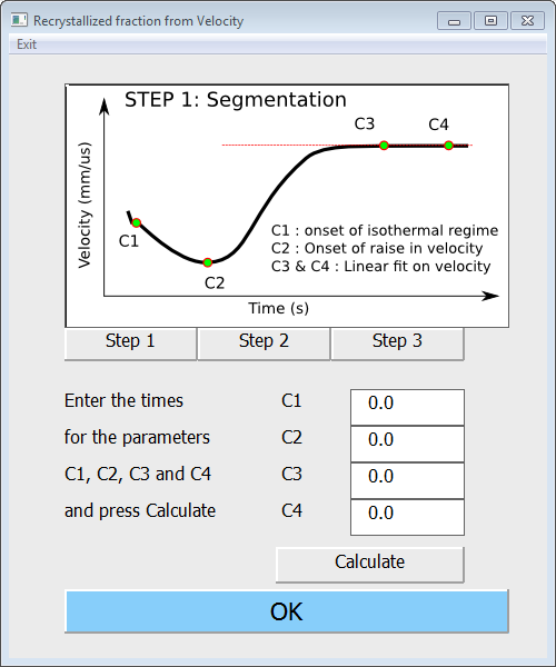
The calculation can be done after entering the four following coefficients.

C1 (s):Time used for the evaluation of the recrystallized fraction from the variation of velocity measured during isothermal holding. C1 is the time at the beginning of the isothermal holding. C2 (s):Time used for the evaluation of the recrystallized fraction from the variation of velocity measured during isothermal holding. The velocity can shows a two step behavior with a minimum present at the beginning of the holding time. C2 is the time at the minimum velocity.

C3 (s):

Time used for the evaluation of the recrystallized fraction from the variation of velocity measured during isothermal holding. At the end of the recrystallization process, the velocity level of to a constant value of velocity. A linear fit is applied on this constant velocity regime. C3 is the low bound of this linear regression.

C4 (s):Time used for the evaluation of the recrystallized fraction from the variation of velocity measured during isothermal holding. At the end of the recrystallization process, the velocity level of to a constant value of velocity. A linear fit is applied on this constant velocity regime. C4 is the low bound of this linear regression.

Once the values are entered in the appropriate boxes, click the button CALCULATE to launch the calculation. The fraction recrystallized is then displayed in the appropriate graph area.